6장 - 이질적 처치효과

6.1 ATE에서 CATE로

Why Prediction is not the Answer

CATE with Regression

import pandas as pd
import numpy as np
from matplotlib import pyplot as plt
import seaborn as sns

import matplotlib

from cycler import cycler

color = ["0.0", "0.4", "0.8"]
default_cycler = cycler(color=color)
linestyle = ["-", "--", ":", "-."]
marker = ["o", "v", "d", "p"]

plt.rc("axes", prop_cycle=default_cycler)

matplotlib.rcParams.update({"font.size": 18})

data = pd.read_csv("../data/daily_restaurant_sales.csv")

data.head()

	rest_id	day	month	weekday	weekend	is_holiday	is_dec	is_nov	competitors_price	discounts	sales
0	0	2016-01-01	1	4	False	True	False	False	2.88	0	79.0
1	0	2016-01-02	1	5	True	False	False	False	2.64	0	57.0
2	0	2016-01-03	1	6	True	False	False	False	2.08	5	294.0
3	0	2016-01-04	1	0	False	False	False	False	3.37	15	676.5
4	0	2016-01-05	1	1	False	False	False	False	3.79	0	66.0

import statsmodels.formula.api as smf

X = ["C(month)", "C(weekday)", "is_holiday", "competitors_price"]
regr_cate = smf.ols(f"sales ~ discounts*({'+'.join(X)})", data=data).fit()

ols_cate_pred = regr_cate.predict(
    data.assign(discounts=data["discounts"] + 1)
) - regr_cate.predict(data)

Evaluating CATE Predictions

train = data.query("day<'2018-01-01'")
test = data.query("day>='2018-01-01'")

X = ["C(month)", "C(weekday)", "is_holiday", "competitors_price"]
regr_model = smf.ols(f"sales ~ discounts*({'+'.join(X)})", data=train).fit()

cate_pred = regr_model.predict(
    test.assign(discounts=test["discounts"] + 1)
) - regr_model.predict(test)

from sklearn.ensemble import GradientBoostingRegressor

X = ["month", "weekday", "is_holiday", "competitors_price", "discounts"]
y = "sales"

np.random.seed(42)
ml_model = GradientBoostingRegressor(n_estimators=50).fit(train[X], train[y])

ml_pred = ml_model.predict(test[X])

np.random.seed(123)

test_pred = test.assign(
    ml_pred=ml_pred,
    cate_pred=cate_pred,
    rand_m_pred=np.random.uniform(-1, 1, len(test)),
)

test_pred[["rest_id", "day", "sales", "ml_pred", "cate_pred", "rand_m_pred"]].head()

	rest_id	day	sales	ml_pred	cate_pred	rand_m_pred
731	0	2018-01-01	251.5	236.312960	41.355802	0.392938
732	0	2018-01-02	541.0	470.218050	44.743887	-0.427721
733	0	2018-01-03	431.0	429.180652	39.783798	-0.546297
734	0	2018-01-04	760.0	769.159322	40.770278	0.102630
735	0	2018-01-05	78.0	83.426070	40.666949	0.438938

Effect by Model Quantile

from toolz import curry


@curry
def effect(data, y, t):
    return np.sum((data[t] - data[t].mean()) * data[y]) / np.sum(
        (data[t] - data[t].mean()) ** 2
    )

effect(test, "sales", "discounts")

32.16196368039615

def effect_by_quantile(df, pred, y, t, q=10):
    # makes quantile partitions
    groups = np.round(pd.IntervalIndex(pd.qcut(df[pred], q=q)).mid, 2)

    return (
        df.assign(**{f"{pred}_quantile": groups})
        .groupby(f"{pred}_quantile")
        # estimate the effect on each quantile
        .apply(effect(y=y, t=t))
    )


effect_by_quantile(test_pred, "cate_pred", y="sales", t="discounts")

cate_pred_quantile
17.50    20.494153
23.93    24.782101
26.85    27.494156
28.95    28.833993
30.81    29.604257
32.68    32.216500
34.65    35.889459
36.75    36.846889
39.40    39.125449
47.36    44.272549
dtype: float64

import warnings

warnings.filterwarnings("ignore")

fig, axs = plt.subplots(1, 3, sharey=True, figsize=(15, 4))
for m, ax in zip(["rand_m_pred", "ml_pred", "cate_pred"], axs):
    effect_by_quantile(test_pred, m, "sales", "discounts").plot.bar(ax=ax)
    ax.set_ylabel("Effect")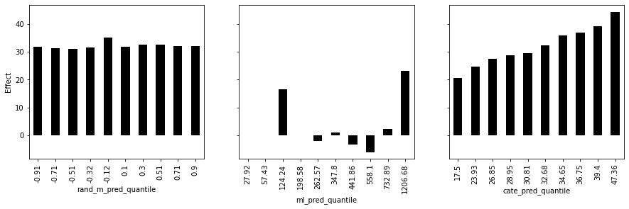

Cumulative Effect

np.set_printoptions(linewidth=80, threshold=10)

def cumulative_effect_curve(dataset, prediction, y, t, ascending=False, steps=100):
    size = len(dataset)
    ordered_df = dataset.sort_values(prediction, ascending=ascending).reset_index(
        drop=True
    )

    steps = np.linspace(size / steps, size, steps).round(0)

    return np.array(
        [effect(ordered_df.query(f"index<={row}"), t=t, y=y) for row in steps]
    )


cumulative_effect_curve(test_pred, "cate_pred", "sales", "discounts")

array([49.65116279, 49.37712454, 46.20360341, ..., 32.46981935, 32.33428884,
       32.16196368])

plt.figure(figsize=(10, 4))

for m in ["rand_m_pred", "ml_pred", "cate_pred"]:
    cumu_effect = cumulative_effect_curve(test_pred, m, "sales", "discounts", steps=100)
    x = np.array(range(len(cumu_effect)))
    plt.plot(100 * (x / x.max()), cumu_effect, label=m)

plt.hlines(
    effect(test_pred, "sales", "discounts"),
    0,
    100,
    linestyles="--",
    color="black",
    label="Avg. Effect.",
)
plt.xlabel("Top %")
plt.ylabel("Cumulative Effect")
plt.title("Cumulative Effect Curve")
plt.legend(fontsize=14)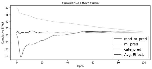

Cumulative Gain

def cumulative_gain_curve(
    df, prediction, y, t, ascending=False, normalize=False, steps=100
):
    effect_fn = effect(t=t, y=y)
    normalizer = effect_fn(df) if normalize else 0

    size = len(df)
    ordered_df = df.sort_values(prediction, ascending=ascending).reset_index(drop=True)

    steps = np.linspace(size / steps, size, steps).round(0)
    effects = [
        (effect_fn(ordered_df.query(f"index<={row}")) - normalizer) * (row / size)
        for row in steps
    ]

    return np.array([0] + effects)


cumulative_gain_curve(test_pred, "cate_pred", "sales", "discounts")

array([ 0.        ,  0.50387597,  0.982917  , ..., 31.82346463, 32.00615008,
       32.16196368])

fig, (ax1, ax2) = plt.subplots(1, 2, figsize=(15, 5))

for m in ["rand_m_pred", "ml_pred", "cate_pred"]:
    cumu_gain = cumulative_gain_curve(test_pred, m, "sales", "discounts")
    x = np.array(range(len(cumu_gain)))
    ax1.plot(100 * (x / x.max()), cumu_gain, label=m)

ax1.plot(
    [0, 100],
    [0, effect(test_pred, "sales", "discounts")],
    linestyle="--",
    label="Random Model",
    color="black",
)

ax1.set_xlabel("Top %")
ax1.set_ylabel("Cumulative Gain")
ax1.set_title("Cumulative Gain Curve")
ax1.legend()


for m in ["rand_m_pred", "ml_pred", "cate_pred"]:
    cumu_gain = cumulative_gain_curve(
        test_pred, m, "sales", "discounts", normalize=True
    )
    x = np.array(range(len(cumu_gain)))
    ax2.plot(100 * (x / x.max()), cumu_gain, label=m)

ax2.hlines(0, 0, 100, linestyle="--", label="Random Model", color="black")

ax2.set_xlabel("Top %")
ax2.set_ylabel("Cumulative Gain")
ax2.set_title("Cumulative Gain Curve (Normalized)")

Text(0.5, 1.0, 'Cumulative Gain Curve (Normalized)')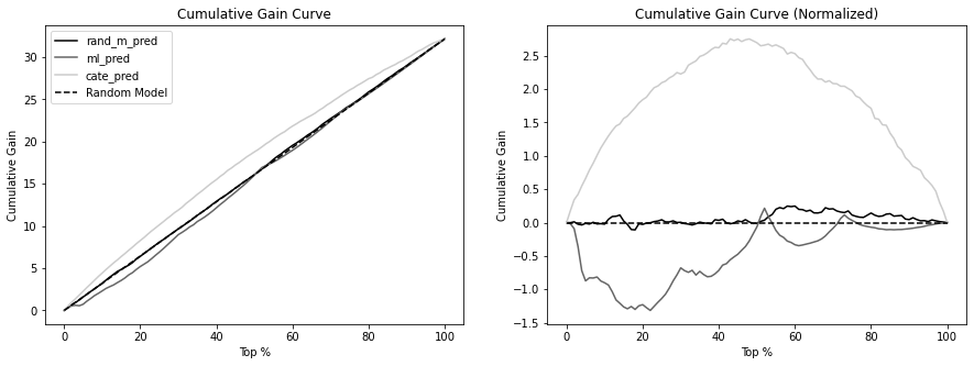

for m in ["rand_m_pred", "ml_pred", "cate_pred"]:
    gain = cumulative_gain_curve(test_pred, m, "sales", "discounts", normalize=True)
    print(f"AUC for {m}:", sum(gain))

AUC for rand_m_pred: 6.0745233598544495
AUC for ml_pred: -45.44063124684
AUC for cate_pred: 181.74573239200615

Target Transformation

X = ["C(month)", "C(weekday)", "is_holiday", "competitors_price"]

y_res = smf.ols(f"sales ~ {'+'.join(X)}", data=test).fit().resid
t_res = smf.ols(f"discounts ~ {'+'.join(X)}", data=test).fit().resid

tau_hat = y_res / t_res

from sklearn.metrics import mean_squared_error

for m in ["rand_m_pred", "ml_pred", "cate_pred"]:
    wmse = mean_squared_error(tau_hat, test_pred[m], sample_weight=t_res**2)
    print(f"MSE for {m}:", wmse)

MSE for rand_m_pred: 1115.803515760459
MSE for ml_pred: 576256.7425385397
MSE for cate_pred: 42.90447405550281

When Prediction Models are Good for Effect Ordering

Marginal Decreasing Returns

np.random.seed(123)

n = 1000
t = np.random.uniform(1, 30, size=n)
y = np.random.normal(10 + 3 * np.log(t), size=n)

plt.figure(figsize=(10, 4))
plt.scatter(t, y)
plt.ylabel("Y")
plt.xlabel("T")

Text(0.5, 0, 'T')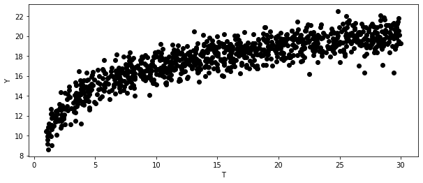

Binary Outcomes

np.random.seed(123)

fig, (ax1, ax2, ax3) = plt.subplots(1, 3, figsize=(15, 5))

n = 10000
t = np.random.uniform(1, 30, size=n).round(1)
y = (np.random.normal(t, 5, size=n) > 15).astype(int)

df_sim = pd.DataFrame(dict(t=t, y=y)).groupby("t")["y"].mean().reset_index()
df_sim

ax1.scatter(df_sim["t"], df_sim["y"])
ax1.set_ylabel("Y")
ax1.set_xlabel("T")


n = 10000
t = np.random.exponential(1, n).round(1).clip(0, 8)
y = (np.random.normal(t, 2, size=n) > 6).astype(int)

df_sim = (
    pd.DataFrame(dict(t=t, y=y, size=1))
    .query("t<6")
    .groupby("t")
    .agg({"y": "mean", "size": "sum"})
    .reset_index()
)

sns.scatterplot(data=df_sim, y="y", x="t", size="size", ax=ax2, sizes=(5, 100))
ax2.set_ylabel("Default Prob.")
ax2.set_xlabel("Loan (in 100k)")


n = 10000
t = np.random.beta(2, 2, n).round(2) * 10
y = (np.random.normal(5 + t, 4, size=n) > 0).astype(int)

df_sim = (
    pd.DataFrame(dict(t=t, y=y, size=1))
    .groupby("t")
    .agg({"y": "mean", "size": "sum"})
    .reset_index()
)

sns.scatterplot(data=df_sim, y="y", x="t", size="size", ax=ax3, sizes=(5, 100))
ax3.set_ylabel("Conversion")
ax3.set_xlabel("Discount (%)")
plt.tight_layout()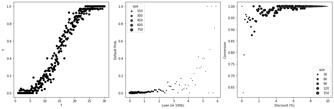

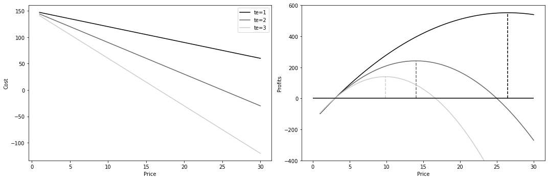
CATE for Decision Making

def demand(price, tau):
    return 50 - tau * price


fig, (ax1, ax2) = plt.subplots(1, 2, figsize=(15, 5))

prices = np.linspace(1, 15)

for i, tau in enumerate([1, 2, 3]):
    q = demand(prices, tau)
    ax1.plot(prices, q, color=f"C{i}", label=f"te={tau}")
    ax2.plot(prices, q * prices, color=f"C{i}", label=f"te={tau}")

ax1.set_ylabel("Demand")
ax1.set_xlabel("Price")

ax2.set_ylabel("Revenues")
ax2.set_xlabel("Price")

ax1.legend()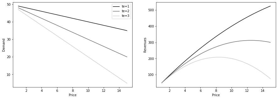

def cost(q):
    return q * 3


def profit(price, tau):
    q = demand(price, tau)
    return q * price - cost(q)


prices = np.linspace(1, 30)

fig, (ax1, ax2) = plt.subplots(1, 2, figsize=(15, 5))

for i, tau in enumerate([1, 2, 3]):
    profits = profit(prices, tau)

    max_price = prices[np.argmax(profits)]

    ax1.plot(prices, cost(demand(prices, tau)), label=f"te={tau}")

    ax2.plot(prices, profits, color=f"C{i}", label=f"te={tau}")
    ax2.vlines(max_price, 0, max(profits), color=f"C{i}", linestyle="--")
    ax2.set_ylim(-400, 600)


ax2.hlines(0, 0, max(prices), color="black")
# ax2.legend()
ax2.set_ylabel("Profits")
ax2.set_xlabel("Price")
ax1.legend()
ax1.set_ylabel("Cost")
ax1.set_xlabel("Price")

plt.tight_layout()

Key Ideas